Methodology

The World Emissions Clock (WEC) provides information about sectoral Greenhouse Gas (GHG) emissions for three different potential futures–one depicting business as usual, one assuming the full implementation of countries’ (or regions’) Nationally Determined Contributions (NDCs), and one depicting a globally cost-efficient way of limiting global warming to 1.5°C compared to pre-industrial levels. For these scenarios, GHG pathways of individual sectors within countries are provided, covering a global sample of 182 countries, with up to 24 subsectors within each country and up to the year 2050. Several parts of the methodology behind the World Emissions Clock have been published in academic journals or are in the process of peer review in the academic community.

Out of the three scenarios, two depict ones that take policy changes explicitly into account. The first scenario gauges future GHG emissions where countries (or regions) fully implement their pledged policies and measures as written down in their NDCs submitted to the United Nations Framework Convention on Climate Change (UNFCCC). While NDCs are mostly submitted by individual countries, there are also ones that are submitted by supranational bodies. For example, the European Union submits its NDC on behalf of its member states, which is also the one reflected on the World Emissions Clock. Some countries within the European Union have more ambitious climate goals, these are not reflected in order to retain consistency across countries. The second scenario shows pathways of necessary GHG reductions in order to limit global warming to less than 1.5°C. Underlying this scenario is a global economic efficiency perspective that yields pathways reflecting the most cost-effective way to meet the Paris goals.

The trajectories of GHG emissions under these two scenarios are provided by the International Institute for Applied Systems Analysis (IIASA) and are based on global Integrated Assessment Models (IAMs) applied under the NGFS project (Bertram et al, 2021; Richters et al, 2022; Richters et al, 2025). The NGFS Climate Scenarios explore a broad range of plausible outcomes for GHG emissions and other indicators under different scenarios, building on different assumptions about the implementation of future climate policies and technological advances on a world region scale. Established downscaling methods, similar to those described in Sferra et al (2021), are then used to break regional results derived from the global IAMs down to the country level utilizing country-level information about the energy mix, development status, and other relevant variables describing the demographics of a country for a given base year. The future evolution of sectoral GHG emissions is then derived by building on assumptions and established projections of the development of these indicators, the so-called Shared Socioeconomic Pathways (SSPs), and their translation into GHGs. There is a range of different IAMs used by the climate science community, differing in their model structure and assumptions, potentially providing different projected pathways of GHGs for a similar scenario with respect to outcomes (e.g., global warming of 1.5°C by 2100). For the sake of simplicity, the WEC only shows one such pathway for each of the two scenarios chosen. For CO₂ emissions derived from the MESSAGE-GLOBIOM model (Huppmann et al, 2019), downscaled to the country level (Sferra et al, 2021), and for non-CO₂ GHG emissions from the GAINS model (Höglund-Isaksson et al, 2020; Winiwarter et al, 2018; Purohit et al, 2020; Gomez-Sanabria et al, 2022); both models are run by IIASA.

The cost-efficiency perspective that the scenario limiting global warming to 1.5°C until 2100 is built on implies that the derived pathways do not incorporate a fair share perspective based on the development status or cumulative emissions of a given country. It is important to note that the modelled pathways are thus not suitable to formulate fair share targets, neither on the aggregate nor on the sectoral level. For a detailed discussion about fair share targets and modelled pathways consistent with such a notion, we refer to the Climate Action Tracker that provides detailed analyses on the aggregate level for a limited subset of countries in this regard.

It should also be noted that there are several scenarios with different pathways that are compatible with meeting the Paris goal of limiting global warming to 1.5°C compared to pre-industrial times or how measures defined in the NDC of a country affect GHG emissions. These scenarios differ in their assumptions about technological change, for example in the take up of technologies for carbon capture and storage (see carbon sinks in the glossary). Depending on these assumptions, scenarios can include GHG pathways that allow for a temporary overshoot of temperatures before 2100 that are offset in later decades by removing carbon from the atmosphere. Similarly, there are a range of IAMs that compute scenario trajectories and they also differ in their assumptions and how they are solved. This also introduces uncertainties about the specific pathway to reach the Paris goals. It is important to acknowledge that considerable uncertainty about the scenarios and their implied pathways exists. These uncertainties stem from the structure of the models they are derived from but importantly also from unknown feedback loops and reinforcing mechanisms of GHG emissions and their effects. The WEC abstracts from these uncertainties to retain an easy-to-use and accessible interface. For a more detailed discussion and view about these uncertainties for a limited set of countries, we refer to the 1.5°C national pathway explorer developed and run by Climate Analytics. Similarly, there are different ways to incorporate the NDCs submitted by parties to the UNFCCC, depending on their formulation. For the WEC, only unconditional NDCs are reflected, which are ones that reflect what countries are pledging to do without international means of support. Relatedly, when an NDC is submitted by a supranational organisation (as is the case for the European Union and its member states), there might be more ambitious climate plans pursued by individual members in addition to the NDC. These more stringent action plans (for example, the new German Climate Protection Act) are not reflected in the respective pathways to retain consistency across countries from a global perspective.

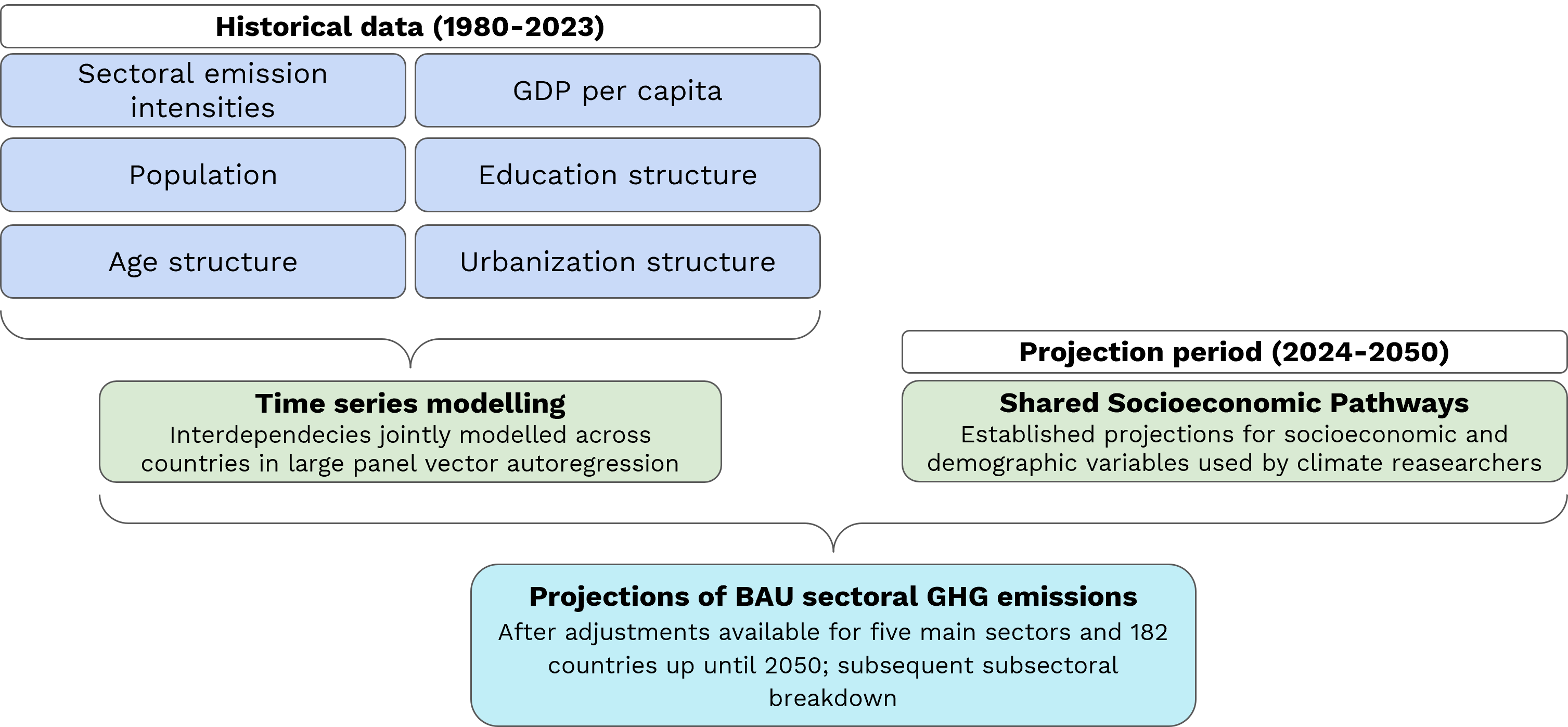
The third scenario depicts a business as usual case. World Data Lab developed the methodology behind this scenario in close cooperation with its academic partners at the Vienna University of Economics and Business (WU Wien), University of Oxford and IIASA. Projections of GHGs in this scenario are based on past interdependencies between the main drivers of overall emissions on a national scale: population, affluence–as measured by Gross Domestic Product (GDP) per capita–, and technology. Technology is defined as the emission intensity in a given sector, i.e. how many tons of GHGs are emitted to produce a given unit of GDP. The main drivers are supplemented by information on demographics of a given country (i.e. age and education structure) as well as on its urbanisation structure. Figure 1 gives an overview of the approach.

To derive sector- and country-specific estimates about interdependencies between included variables large time series models were employed. Changes in technology and policy-making reflected as changes in GHG emission intensities are projected forward using information about past interdependencies and trends. This abstracts from making assumptions about future policy actions but models them explicitly based on past actions. By modelling sectoral emission intensities instead of GHG emissions directly, we capture the notion of technology and policy changes in a given sector and country. However, progress in technology may not always translate into reduced emissions. In particular, if population and GDP increases exceed the reduction of emission intensity, we may still see rising emissions in this country and sector. Future trends, based on past experience, are based on and complemented by established projections of socioeconomic variables as derived from the Shared Socioeconomic Pathways (SSPs) and short-term economic changes as implied by GDP forecasts by the International Monetary Fund. Using this information, we compute the evolution of sectoral GHGs for 182 countries, capturing both short-term fluctuations – for example caused by the disruption of production by the COVID-19 pandemic – and the long-term evolution of GHG emissions for five main sectors of GHG emissions. The breakdown to the subsectoral level is based on information provided by IIASA (see below).

For the projections under a business-as-usual scenario, we rely upon publicly available datasets. For historical information on sectoral GHG emissions, we use the comprehensive and detailed database provided by Minx et al. (2021). It is based on the Emissions Database for Global Atmospheric Research (EDGAR) of the European Commission and captures emissions for over 200 countries and territories, differentiated by five main sectors and more than 60 subsectors. It is important to note that due to the global nature of EDGAR and derived products, such as the database of Minx et al. (2021), implies that historical observations of emissions, and thus also starting levels for the projected evolution of them, might deviate from those reported from countries in their official documents. This is especially the case for countries where reporting guidelines are non-standardized in contrast to those countries that have to provide annual GHG inventories to the UNFCC, the so-called Annex I Parties. Thus, for countries with limited capacities, such as ones from the Global South, deviations from country reports might be larger. However, the standardized and independent nature of EDGAR increases the comparability of data across countries and time periods immensely.

Historical data on GDP and population sizes are taken from various sources such as the World Development Indicators of the World Bank and imputations are carried out for countries with missing data. Additional data describing the demographic structure of countries are sourced from the Wittgenstein Centre for Demography and Global Human Capital, the World Urbanization Prospects of the United Nations and other scientific studies (e.g. SSP-consistent projections for urbanisation are taken from Chen et al, 2022). For the projection period, we use projections of variables consistent with the SSP2 scenario, which describes a “Middle of the Road” case in terms of human development and demographic changes up until 2100.

For a small number of country-sector pairs the time series model yielded unrealistic forecasts of emission intensities, typically resulting in exceedingly high sectoral emission forecasts. Where this was the case, ex-post adjustments were necessary. In particular, the evolution of sectoral emission intensities in geographically neighbouring countries were used as information to adjust forecasts, starting from the last observed time period. The same was done to extend the sample for a small number of countries not included in the modelling exercise due to missing data. Given their high variability, conceptual differences, and distinct nature in key drivers, land use, land use change and forestry (LULUCF) emissions were not included in this forecasting exercise but rather derived by downscaling regional projections from the MESSAGE-GLOBIOM model (Huppmann et al 2019) provided by IIASA using historical information from country-reported values (see below).

Figure 1: Schematic overview of procedure for deriving BAU GHG emissions projections

Necessary adjustments/expansions:

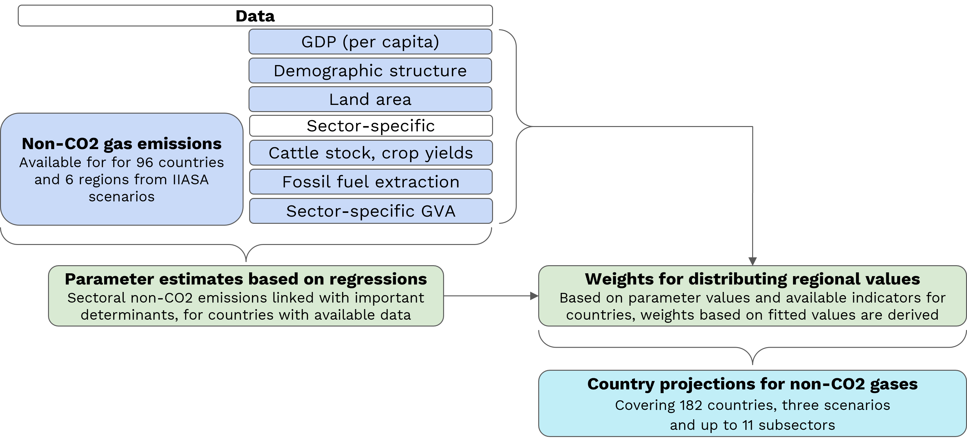
Some ex-ante adjustments were necessary to expand parts of the data provided by IIASA. For the non-CO₂ gases, information about the NDC and 1.5°C scenario GHG trajectories are available only at the regional level for certain parts of the sample (e.g., a “North Africa” region comprising Algeria, Libya, Morocco and Tunisia), whereas for other countries they were readily available. To break these data down to the country level, we used regressions for those countries where information was available to derive parameter estimates for important drivers of emissions in a certain subsector (e.g., the amount of cattle in a country as a determinant of emissions in the livestock sector). Using these parameter estimates, we calculated shares of regional emissions to be attributed to countries in this region. Comparisons with historical data showed that this approach yields satisfactory alignment for a number of comparison years. Using information about the projected evolution of non-CO₂ gas emissions on a regional level from IIASA and these estimated shares, projected emissions on the regional level were distributed to country level in a similar fashion. Figure 2 gives an overview of the necessary steps.

Figure 2: Schematic overview of procedure to break down regional non-CO₂ gas pathways to country level

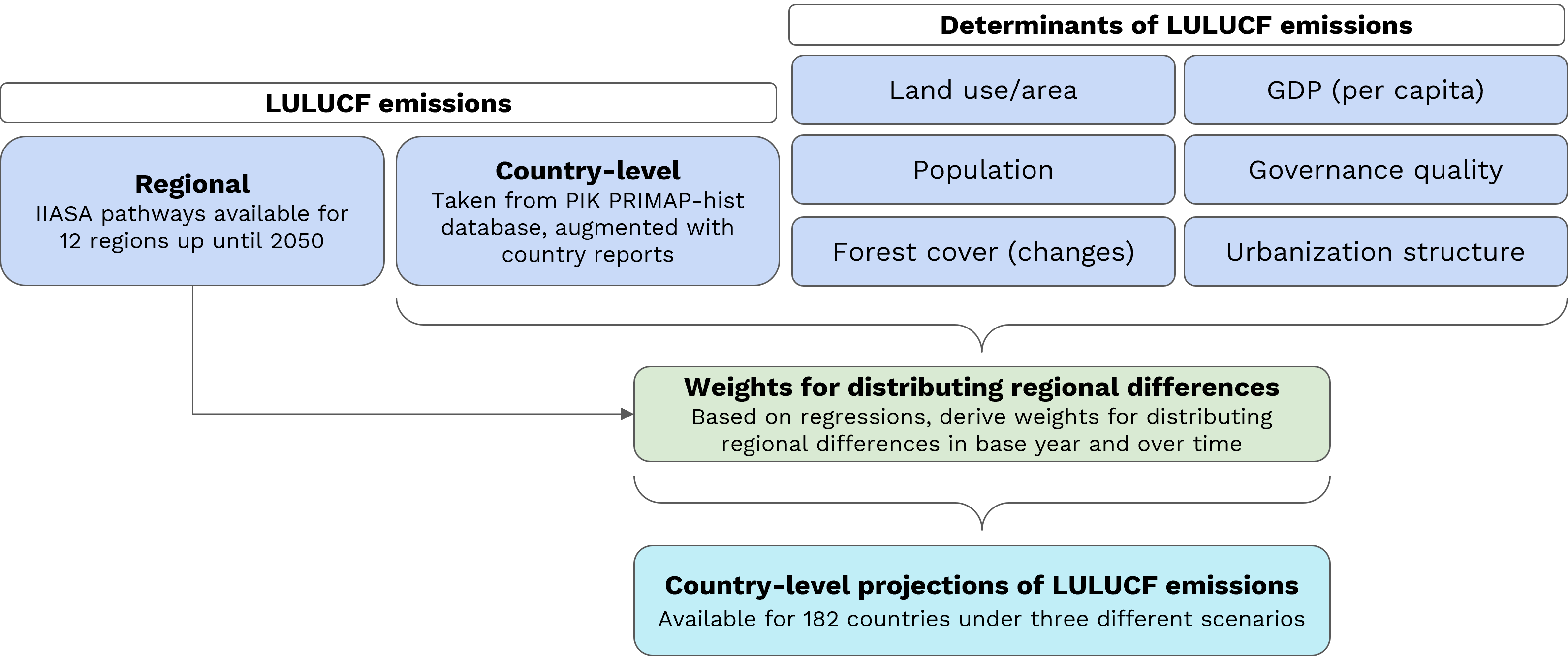
A special case arises for emissions from LULUCF. There are conceptual differences between country reports and results from global Integrated Assessment Models (IAMs), see e.g. Grassi et al (2018), Grassi et al (2021). To overcome these differences, we adjust country-reported values such that regional sums correspond to those derived by IAMs. We use a regression-based approach linking LULUCF emission values as reported in the PIK PRIMAP-hist database in a base year to potential drivers such GDP, population, forest cover and governance indicators, among others. Based on squared predicted values from these regressions, we constructed weights to distribute the differences in regional emissions. Going forward in time, we constructed weights based on the parameter estimates from these regressions updated with variable values implied by projections consistent with the Shared Socioeconomic Pathways (SSPs). These weights are then used to distribute changes in emissions implied by regional pathways. This way countries that have a large potential for emissions in this sector-but conversely also large potential for reductions therein-get attributed a larger share of the changes over time implied by the regional results. Validation exercises with expert-based assessments of LULUCF emissions for a set of 20 countries world-wide yielded good agreement, both in terms of levels in the base year as well as in terms of dynamics over time. However, it should be stressed that the adjustment carried out makes comparisons with other, existing LULUCF datasets cumbersome. Given the large uncertainties about LULUCF emissions and conceptual differences in their accounting by countries, they should be viewed with caution. We strive to continuously update the data underlying the adjustment in close contact with country governments as information on this sector grows. Figure 3 gives an overview of the used approach.

Figure 3: Schematic overview of procedure for deriving country-level LULUCF emission pathways

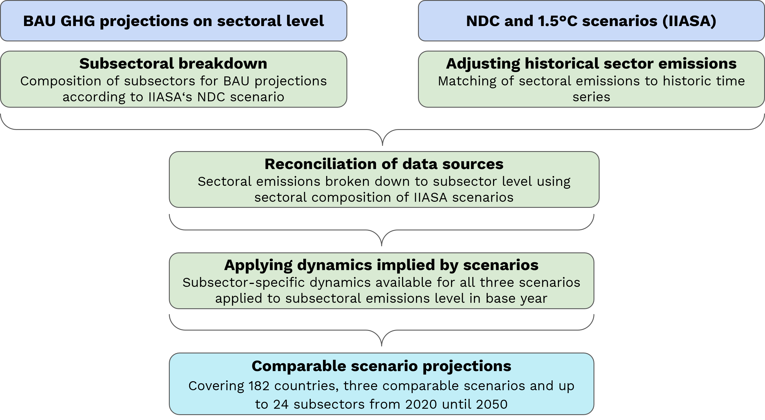
Given the different data sources for GHG emissions under different scenarios, some harmonisation across them was required. Data on the sectoral level prior to 2022 are consistent with the historically available data provided from the database by Minx et al. (2021), and with dynamics from the EDGAR database for the years 2022 and 2023. After that predictions of the time series model are used. The year 2023 serves as an anchor from which onwards the evolution of sectoral GHG emissions implied by the NDC and 1.5°C scenarios are applied to. In combination with the trajectory derived from the time series model, this yields comparable pathways for the three scenarios. For the subsectoral composition of the business-as-usual scenario the shares of the individual subsectors as implied from the IIASA’s NDC trajectory were computed in each year and country. These shares were then used to break down the projections yielded for the five main sectors from the time series econometric approach. Figure 4 gives an overview of the reconciliation process.

Figure 4: Schematic overview of data reconciliation across sources and scenarios

After all adjustments and reconciliation across sources, the WEC covers 182 countries worldwide and up to 24 sectors per country up to the year 2050. In addition it covers emissions from international aviation and shipping as separate categories. Considering all three scenarios across all countries, more than 12,000 trajectories for sectoral GHG emissions are considered. This extensive coverage allows for comparisons of GHG emissions trajectories across countries, sectors, and time.

Abbreviations

GHG - Greenhouse gases

CO₂eq - CO₂ equivalents

GT - Gigaton

MT - Megaton

KT - Kiloton

s / sec - Second

GDP - Gross domestic product

IPCC - Intergovernmental Panel on Climate Change

NDC - Nationally Determined Contributions

SSP - Shared Socioeconomic Pathways

COP - Conference of the Parties

LULUCF - Land use, land use change and forestry

Glossary

Greenhouse Gases (GHG) – Captures all gases that are recognized in the Kyoto protocol to cause climate change and related global warming. They include carbon dioxide (CO₂), methane (CH₄), nitrous oxide (N₂O), and a range of F-gases such as Hydrofluorocarbons (HFCs) or Perfluorocarbons (PFCs).

Non-CO₂ gases – All greenhouse gases except carbon dioxide.

CO₂ equivalents (CO₂eq) – A metric measure that is used to compare emissions from various greenhouse gases, converting amounts of non-CO₂ greenhouse gases into the equivalent amount of CO₂ with the same global warming potential.

Global warming potential – Different greenhouse gases have different potencies with regards to their contribution to global warming and their longevity in the atmosphere. Global warming potentials are used to convert non-CO₂ gases into CO₂ equivalents, taking CO₂ as the gas of reference with a global warming potential of 1. The WEC expresses greenhouse gases in global warming potentials calculated over 100 years.

Carbon budget – Refers to the maximum of cumulative net CO₂ emissions that would result in limiting global warming to a given level with a given probability. While it excludes non-CO₂ gases, it takes into account their effects regarding their potential for global warming. It provides a simple number to express how much CO₂ can still be emitted before a desired global temperature increase is exceeded. In the WEC, we take the cumulative sum of the 1.5°C scenario as the carbon budget. However, please note that there are several pathways towards limiting temperature increases to 1.5°C compared to pre-industrial times and results also differ across different Integrated Assessment models.

Gigaton (GT) – One billion tons of greenhouse gas emissions CO₂ equivalents.

Megaton (MT) – One million tons of greenhouse gas emissions in CO₂ equivalents.

Kiloton (KT) – One billion tons of greenhouse gas emissions in CO₂ equivalents.

Land use, land use change and forestry (LULUCF) – This category refers to emissions from land use, land use change and forestry that stem from the impact of humans on terrestrial carbon sinks. While it includes a range of different types of land use (change), including for example conversion of grassland to cropland, by far the largest contribution is attributed to changes in forests. Activities in this sector can either act as carbon sources (e.g. through deforestation) or as carbon sinks (e.g. through afforestation). Note that there are conceptual differences in the accounting of emissions in this sector, causing large variations across data sources and large uncertainties.

Carbon sink – Refers to anything that absorbs more greenhouse gases from the atmosphere than it emits. Natural carbon sinks include the oceans, forests (or other vegetation) and the soil. While the development of artificial (i.e. non-natural) carbon sinks, often referred to as carbon capture and storage solutions, is still in its infancy, their wide-spread adoption in the future is viewed as an important way for mitigation.

Carbon neutrality – Describes a situation where emissions caused by humans are balanced with their removals, e.g. through afforestation or non-natural carbon sinks, or are eliminated altogether. Although the term refers to CO₂ only, it typically also includes other GHGs.

Integrated Assessment Models (IAMs) – Models used in the climate science community to understand and assess how choices about human development and society affect each other and repercussions on the environment, including climate change. They incorporate and/or model certain assumptions about the future availability and adoption of energy technologies, energy use, land use changes and societal trends that influence GHG emissions.

Downscaling – Refers generally to procedures that are used to break down global or regional emission pathways to the country and/or sectoral level.

United Nations Framework Convention on Climate Change (UNFCCC) – The body of the United Nations that was established to combat “dangerous human interference with the climate system”. Established in 1992, and adopted in multiple rounds (most notably with the Paris Agreement in 2015), it sets out basic legal framework and principles for international climate change cooperation. This includes measures planned by participating parties as part of their Nationally Determined Contributions (NDCs) as well as reporting on GHG emissions under a common reporting principle.

Nationally Determined Contributions (NDCs) – Non-binding plans of parties to the UNFCCC detailing actions and targets for climate change mitigation. Most importantly, they include targets for the reduction of greenhouse gas emissions as well as measures and policies to achieve these targets as a contribution to achieve the goals of the Paris agreement.

Conference of the Parties (COP) – Annual climate change conference of the parties to the UNFCCC to assess progress and setbacks as well as negotiating agreements for dealing with climate change, taking place in different cities every year.

Paris agreement – Legally binding international treaty on climate change and ways to combat it adopted in 2015 as a result of COP21 taking place in Paris, entering force in 2016. Adopted by 196 parties to the UNFCCC, its goal is to limit global warming in 2100 to 2° Celsius, preferably 1.5°C, compared to pre-industrial times. This is to be achieved by striving for reaching global peaking GHG emissions as soon as possible and achieving global carbon neutrality by mid-century.

Shared Socioeconomic Pathways (SSPs) – Depict different scenarios of the development of global socioeconomic changes for a variety of variables, typically up to the year 2100. They are often used as inputs for IAMs to derive greenhouse gas emissions scenarios and explore difference climate pathways.

Time series model – Refers to a class of models where present values of certain variables are related to their lagged values, i.e. their past realizations, as well as to lagged values of other variables.

Gross domestic product (GDP) – Measure for the value added created through the production of goods and services within a certain country and time period (typically within a year).

Sector and scenario definitions

Sectoral composition – The WEC classifies greenhouse gas emissions by five main sectors–energy systems, industry, agriculture, transport, and buildings–and up to 24 subsectors per country. Emissions caused by international shipping are captured in a separate category as they cannot be meaningfully assigned to an individual country.

Agriculture – Captures emissions from the cultivation of crops, the keeping of livestock, and those caused by land use change. The latter refers to emissions caused mostly by forest clearing and deforestation but also captures other land use changes, e.g. the conversion from grass- and bushland to farmland.

Crops - Includes emissions from the application of mineral and natural (manure) fertilizers on soils and pasture, open burning of field residuals, and rice cultivation.
Livestock - Includes emissions from manure management and the enteric fermentation of the digestive process in ruminant animals such as cattle, sheep or goats.
Land use change - Includes emissions from land use, land use change and forestry.

Industry – Captures emissions caused by different industrial sectors, including those caused by burning fossil fuels and those arising as a side-product from industrial processes (e.g. oxidisation in the in the production process of cement), as well as those caused by the processing and disposal of waste. Note that the country perspective might deflect from heterogeneity of firms within a given sector, with some being less carbon-intensive than others.

Metals - Includes emissions from the production and processing of ferrous and non-ferrous metals, blast furnaces and industrial processes involved.
Chemicals - Includes emissions from the production of chemicals but also glass and lime production.
Cement - Includes emissions from the production of cement.
Other (industry) - Includes emissions from industries such as pulp and paper production, food processing, machinery construction or textiles, among others.
Waste - Includes emissions from waste disposal on landfills, waste treatment through composting and biodigestion, and incineration as well as centralised wastewater management for industries and buildings.

Energy (systems) – Captures emissions from electricity production (including from coal, gas, oil) and district heating as well as emissions caused by the extraction and production of fossil fuels (e.g. oil refineries). It furthermore captures also some residual emissions caused by the burning of fossil fuels not captured in any of the other categories.

Electricity production: Coal - Includes emissions caused by the production of electricity in power plants using coal as primary input.
Electricity production: Gas - Includes emissions caused by the production of electricity in power plants using natural gas as primary input.
Electricity production: Oil - Includes emissions caused by the production of electricity in power plants using oil as primary input.
Heating - Includes emissions from centralised heating technologies (as opposed to emissions for decentralised heating in buildings themselves or by industries).
Fossil Fuels Production - Includes emissions from the extraction and conversion of fossil fuels such as coal mining, oil production, and the production and transport of natural gas.
Other Energy Use/Combustion - Includes emissions in the energy-producing sector not captured in the other categories. Acts as a residual for emissions from the burning of fossil fuels not assignable to other emission sources.

Transport – Captures emissions from various modes of transport, including cars and buses/trucks as well as their associated cooling emissions, off-road emissions caused by rail and other transport modes such as pipelines, domestic shipping and air travel, and international shipping emissions.

Cars - Includes emissions from the burning of fossil fuels by passenger cars.
Buses/Trucks - Includes emissions from the burning of fossil fuels by buses and trucks.
Rail and others - Includes emissions from the burning of fossil fuels by rail but also other forms of non-road transport.
Air Travel - Includes emissions from domestic and international aviation.
Ships - Includes emissions from domestic shipping.
Cooling - Includes emissions resulting from leakage in the refrigeration and air conditioning process of road vehicles in the form of F-gases.
International Shipping - Includes emissions from international marine transport. These are captured separately as there exists no general agreement on a methodology for their attribution to individual countries.

Buildings – Captures emissions from heating & cooking in both residential and commercial buildings (including from coal, gas, oil) as well as those caused by cooling buildings (again residential and commercial).

Heating & Cooking: Coal - Includes emissions caused by the burning of coal for heating and cooking in residential and commercial buildings.
Heating & Cooking: Gas - Includes emissions caused by the burning of natural gas for heating and cooking in residential and commercial buildings.
Heating & Cooking: Oil - Includes emissions caused by the burning of oil for heating and cooking in residential and commercial buildings.
Cooling - Includes emissions from the cooling of buildings in the form of leaked F-gases.

Scenarios - The WEC provides information about sectoral GHG emissions for three representative pathways that depict different possible future named “Business as usual”, “Do as we promised”, and “We achieve the goal”. Underlying these scenarios are different assumptions:

Business as usual - Depicts a scenario without drastic deviations in technology advancement or policy-making from past experiences. While there is typically still some technological progress in the form of reducing emissions intensities (stemming e.g. from energy efficiency gains) that are partly a result of policy actions, this scenario does not take into account announced policy pledges.
Do as we promised - Depicts a scenario where countries (or regions) fully implement their announced policies written down in their Nationally Determined Contribution (NDC) submitted to the United Nations Framework Convention on Climate Change (UNFCCC). More ambitious climate action plans pursued by individual countries that are not part of the NDC (of the country itself or the submitting party) are not reflected on the WEC to retain consistency across countries. Hence, here the “we” in “Do as we promised” refers to countries or regions fulfilling their pledges in their NDCs.
We achieve the goal - Depicts a scenario outlining pathways for countries and sectors that are consistent with limiting global warming to 1.5°C compared to pre-industrial times in 2100 as per the Paris agreement from 2015. The trajectories are derived under a global cost efficiency perspective, i.e. they outline the most cost-effective way of achieving the goal of 1.5°C. They are not meant to reflect fair-share considerations based on e.g. cumulative historical emissions. Here, the “we” in “We achieve the goal” refers to the world achieving a global goal.

How to use the WEC and its different pages

Emission (Page 1) – The first page provides an overview of the total amount of greenhouse gases emitted in a certain year until the day the user looks at it. The rotating country-sector combinations exemplify where these emissions are coming from in terms of country and sector. The pairs are chosen at random with underlying probabilities based on the share a certain country-sector pair contributes to global emissions in the selected year. The user can adjust the year for which emissions to date are shown as well as change the underlying scenario. Depending on the amount of overall emissions for a year under a certain scenario, the animation changes to a different speed, to convey the user a sense of urgency for more pessimistic scenarios.

Map (Page 2) – This page lets the user explore emissions by country in an easy manner by simply choosing them either on the map itself or searching for it. Once a country is selected, information about the sectors is provided, sorted from the largest emitting one to the least emitting, together with some relevant statistics for total country emissions. By clicking on one of the sectors, similar information is provided for the subsectors within the sector. The year and scenario for which statistics are shown can be chosen. Users can switch between three views: one showing total emissions per country, one showing emissions per person, and one presenting a classification scheme that categorizes countries by their income and emissions per person. The latter places each country in one of nine quadrants along the dimensions of income (low-middle-high income) and emissions per person (low-medium-high emissions). The income categories are taken from the World Bank and are based on GNI per capita, calculated using the World Bank Atlas method. The income classification of the World Bank is defined for financial years (running from July to June of the subsequent year) as opposed to calendar years. For the sake of simplicity, on the WEC this is adjusted by assuming that the income status of a given calendar year is the one of the subsequent financial year (i.e. for 2023, we take the income classification of the World Bank's 2024 financial year). We project changes in GNI per capita using projected changes in GDP per capita as implied by short-term GDP forecasts by the IMF and projections of the SSP2 scenario. For the emissions classification we use static thresholds of five and ten tons per person for medium and high emitting countries, respectively.

Sectors (Page 3) – This page provides an easy-to-digest overview of sectoral emissions, with countries to be chosen through the search bar and again adjustable by year and scenario. By clicking on the sector icons, more detailed information on the subsectoral composition can be viewed. The view also includes a ranking of per capita emissions, from the least emitting country to the highest emitter (in per capita terms).

Comparison (Page 4) – Currently, this section allows for the comparison of per capita emissions across countries, with information available down to the sectoral level. Future extensions of this section will allow the user to delve into the concepts of implementation and ambition gaps over time for both aggregate and per capita emissions.

What Now (Page 5) – Contains information on the methodology behind the WEC, including a glossary and list of abbreviations, as well as further links to related websites containing information about potential actions to take and what legislators in a given country are proposing.

Common to all subpages of the WEC is the Global Carbon Budget ticker in the top right corner. It shows how much of the remaining carbon budget is left in a given year and scenario or by how much it already was exceeded.

FAQ

What can the World Emissions Clock be used for?

The WEC lends itself to the exploration of GHG emissions pathways in the future on a very detailed, sectoral level. The extensive geographical coverage and consistency in methodology across countries allows for cross-country comparisons including almost every country in the world.

Is the “We achieve the target” scenario based on “fair-share” considerations?

No, this scenario is solely based on a global economic efficiency perspective. This means the depicted pathways in the WEC are computed such that the Paris goal of limiting global warming to 1.5°C compared to pre-industrial times is achieved in the most cost-efficient way from a global point of view. They do not take into account historical emissions and have hence no consideration of “fairness” in terms of burden-sharing incorporated in them. They also make no explicit assumptions about who stems the financial burden of the measures that need to be taken to achieve this goal.

Which country pledges about future actions of countries for emissions mitigation are reflected in the “Do as we promised” scenario?

This scenario incorporates information about measures and pledges written down in the Nationally Determined Contributions that individual countries (or supranational organizations on their behalf) submitted to the United Nations Framework Convention on Climate Change (UNFCCC). It does not, however, include pledges about long-term goals into account that are vaguely formulated and not submitted to the UNFCCC. Similarly, if individual countries for which a supranational organization submitted the NDC on their behalf pursues more ambitious climate action plans, this will not be reflected in this scenario. For example, for member states of the European Union the “Do as we promised” trajectories reflect only those pledges based on the NDC submitted by the European Union to the UNFCCC.

Could actual emissions be different from those reported at the World Emissions Clock?

There is considerable uncertainty surrounding estimates of GHG emissions, especially for non-CO₂ gases such as methane, nitrous oxide and F-gases, or emissions coming from the LULUCF sector. Thus, the numbers the World Emissions Clock provides might indeed differ from other global databases or country reports to a certain extent. We strive to update our underlying data as often as possible to reduce discrepancies, where possible. Additionally, there are different ways to convert emissions of non-CO₂ gases to CO₂ equivalents, depending on the horizon over which they are assumed to absorb energy in the atmosphere. Currently, the World Emissions Clock uses 100-year GWPs to do such a conversion, following common practice. However, one could also use 20-year GWPs, under which current GHG emissions would be considerably higher due to higher conversion rates for short-lived greenhouse gases like methane. Such differences in GWPs used can thus be source of substantial differences but can be adjusted by normalizing across sources.